Motivation

Many students study probability in high school or college but fail to grasp the common-sensical understanding of this natural topic. They usually end up memorising a ton of formulae and applying them to a hundred questions. I don’t know about them, but probability surely deserves better! I will explain everything in granular detail, providing informal, simple explanations alongside formal definitions of various terms and concepts. So, without further ado, let’s start!

The Informal Intro

What is a random variable?

It’s just a function that maps an event’s textual description to a relevant number. For example, if we toss a coin, a random variable \(X\) can be defined as follows:

\[X(heads) = 1\]

Now, let’s toss two coins and define \(X\) to denote the number of heads as shown below:

\[X(TT) = 0\]

So, apparently, the only reason random variables exist is that our X-axis can’t fit words :))! Quite some existential crisis, isn’t it?

What exactly is probability?

Let’s start with the most basic definition of probability. \[probability = \frac {number \, of \, favourable \, outcomes}{total \, number \, of \, possible \, outcomes}\] This can be applied to the simple example of a coin toss using the random variable \(X\)as shown above, as follows: \[prob(X=1) = \frac {1} {2} \, ; \, prob(X=0) = \frac {1} {2}\] However, this definition has two significant limitations :(!

The EQ Problem!

Our definition works well for the unbiased coin toss example. But, let’s take a biased coin with heads on both sides(like the one shown in the movie “Sholay”!). According to our formula: \[prob(X=1) = \frac {num \, outcomes \, having \, heads} {total \, number \, of \, outcomes} = \frac {1}{2}\] However, in reality, \(prob(X=1) = 1\). Hence, our definition does not work when all outcomes are not EQually likely. In such cases, we conduct experiments and note down the outcomes. This gives us the evidence to support our probability values. Hence, the new definition of probability becomes: \[prob(X=\lambda) = \lim\limits_{n_{total} \rightarrow \infty} \frac {n_\lambda} {n_{total}}\] Let’s understand this with the typical example of a coin toss. Suppose we are dumb and don’t know that \(prob(heads) = 0.5\). However, we are not too dumb, so we decided to do ten coin tosses and observe. We get three heads and seven tails. So, we define \(prob(heads) = 0.3\). Now, a moderately clever (but idle!) person says, “Let’s do it 1000 times!”. This time, we get 550 heads and 450 tails. Now, \(prob(heads)\) becomes \(0.55\). As you can notice, as we increase the number of tosses, our probabilities get closer and closer to the correct answer. This is the logic behind the \(n_{total} \rightarrow \infty\) limit in the above formula.

The Infinity Problem

It only works when the total number of possible outcomes is finite. This is a big problem because it is not the case in most practical scenarios. For example, what can we do if we want to find the value of \(prob(temp \in [17.29^{\circ}C, 20^{\circ}C])\) in a room?

Currently, we are viewing probability as just discrete values assigned to a finite number of events. However, think about it and tell me if going around assigning probabilities to each and every point on the x-axis is a good option or not. Of course, it’s foolish. Let’s try peeking through the lens of calculus. One of the main lessons of calculus was to “think in terms of ranges rather than points”. Okay, so we make a graph where the x-axis contains the infinite range of values available to us while the y-axis contains \(prob(X \le x)\). Let’s name this function of this graph as \(cprob\). Hence, rather than focussing on \(prob(X=x)\), we focus on \(prob(X \le x)\). This way, the problem is solved because: \[\small \begin{equation*} \begin{split} prob(temp \in [17.29^{\circ}C, 20^{\circ}C]) &= prob(temp \le 20^{\circ}C) - prob(temp \le 17.29^{\circ}C) \\ &= cprob(temp=20^{\circ}C) - cprob(temp=17.29^{\circ}C) \end{split} \\ \end{equation*}\]

The Functions

Let’s look at some important functions and properties commonly used to define probabilities.

CDF

A cumulative distribution function is a function \(F_X : \mathbb{R} \rightarrow [0, 1]\) which specifies a probability measure as: \[F_X(x) = P(X \le x)\] Some properties of CDF include:

It is an increasing function.
\(lim_{x \rightarrow -\infty} F_X(x) = 0\) as \(P(\phi) = 0\)
\(lim_{x \rightarrow \infty} F_X(x) = 1\) as \(P(\varOmega) = 1\)

PMF

For discrete random variables, it is simpler to literally define the probability for each point. This is called the probability mass function of that random variable. For example, let us consider the tossing of two coins. The random variable is the number of heads, i.e. \(X(\varOmega) \in Val(X) = \{ 0, 1, 2 \}\). So, the PMF \(p_X : Val(X) \rightarrow [0, 1]\) can be defined as follows: \[p_X(0) = 0.25\] \[p_X(1) = 0.5\] \[p_X(2) = 0.25\]

PDF

If a CDF is continuous and differentiable everywhere, the probability density function is defined as the derivative of CDF. \[f_X(x) = \frac{dF_X(x)}{dx}\] Some subtle points about PDFs are as follows:

PDF does not exist for a random variable if its CDF is continuous but not differentiable everywhere.
Value of PDF at a given point \(x\) is not necessarily equal to the probability of that event, i.e.,\[f_X(x) \ne P(X=x)\]In fact, for continuous random variables, \(P(X=x) = 0 \enspace \forall \enspace x\) because we only talk about interval probabilities whenever continuous random variables are concerned.
\(f_X(x) \ge 0\), but not necessarily \(\le 1\), as the derivative can be greater than \(1\).
\(\int_{- \infty}^{\infty} f_X(x) = 1\)

The Properties

Expectation

If \(p_X(x)\) is the PMF of a discrete variable \(X\), \[E[g(X)] = \sum_{x \in Val(X)} g(x)p_X(x)\] On the other hand, for a continuous variable \(X\) with PDF \(f_X(x)\), \[E[g(X)] = \int_{-\infty}^{\infty} g(x)f_X(x)\]

Some properties of expectations are as follows: * \(E[X]\) is the same as \(mean(X)\) conceptually. It’s just that \(E[X]\) is used to define what will happen in the future while \(mean(X)\) is used to “summarise” the past. * \(E[1\{ X=k \}] = P(X=k)\)

Variance

It is the measure of how concentrated a distribution is around its mean. Mathematically, we can express it as: \[Var[X] = E[(X-E[X])^2]\] Also, one more way to write the above formula would be: \[Var[X] = E[X^2] - (E[X])^2\] A simple property of variance is: \[Var[aX] = a^2Var[X]\]

Some Common Probability Distributions

The Discrete Distros

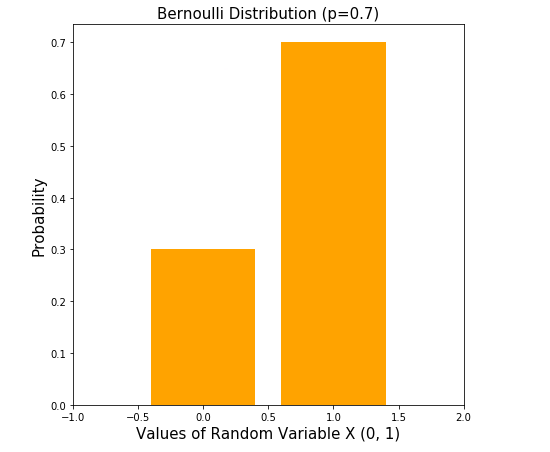
Bernoulli - Probability of getting a head in a simple coin toss!\[\small p_X(x) = \begin{cases} p &\text{if } x = 1 \\ 1 - p &\text{if } x = 0 \end{cases}\]

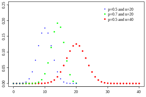
Binomial - Probability of getting \(x\) heads in \(n\) tosses!\[\small p_X(x) = {n \choose x} . p^x (1-p)^{n-x}\]

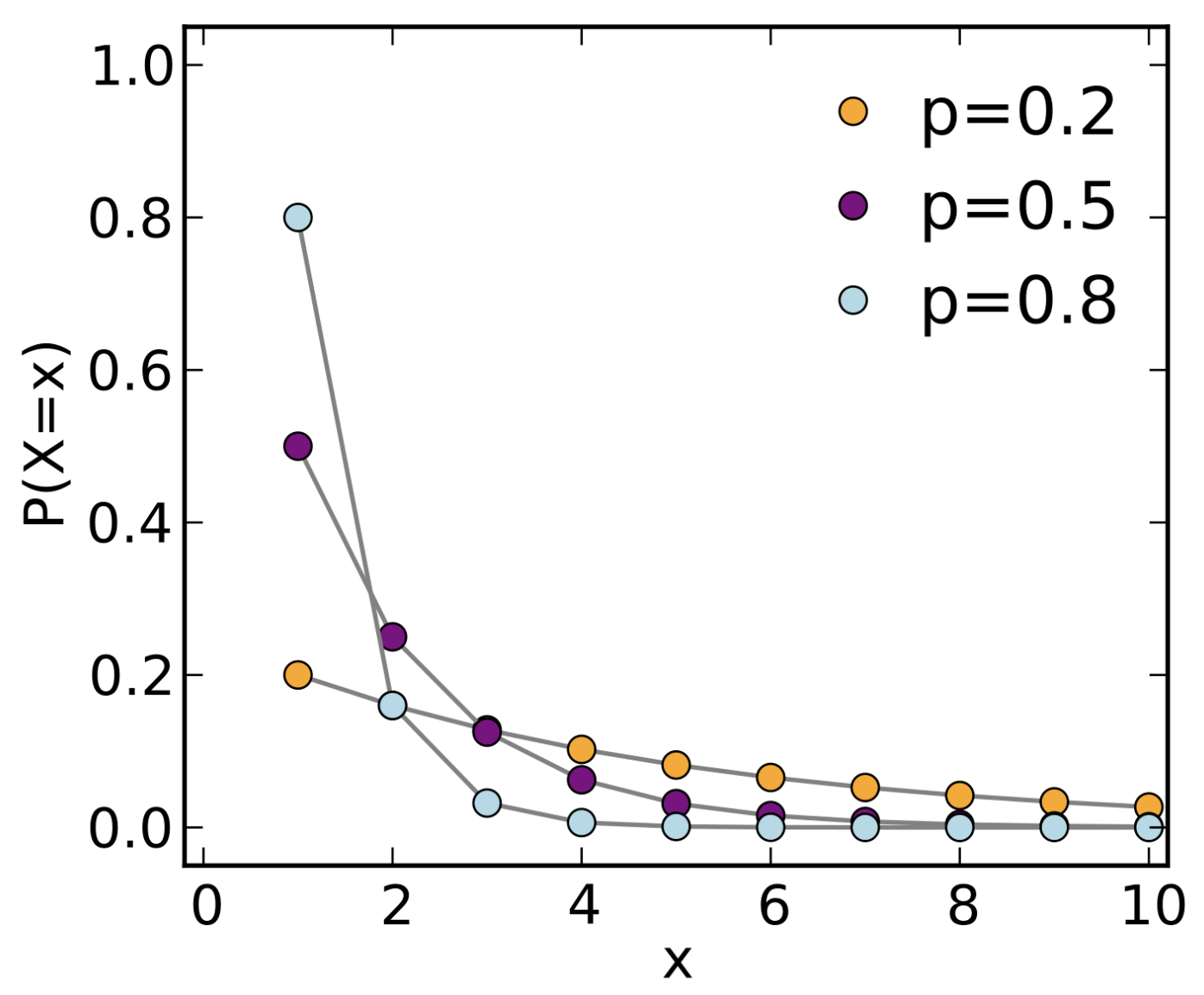
Geometric - Probability of getting the first head at the \(x^{th}\) toss!\[p_X(x) = p(1-p)^{x-1}\]

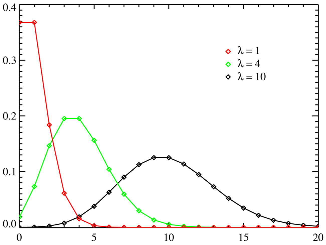
Poisson - It is just a special case of the binomial distribution but requires some further explanation. In binomial, we know the number of trials and the probability of success in a particular trial. However, imagine a situation where we know the average success rate over a given period. Let this rate of success be \(\lambda\). Also, the number of trials \(n\) would tend to \(\infty\). Put \(p = \frac {\lambda} {n}\) in the binomial formula. After solving the limit on \(n \rightarrow \infty\) (full proof here), we get the following formula to find out the probability of getting \(k\) successes per period (the same as \(\lambda\)’s period) would be:\[p_X(X=k) = \frac {e^{-\lambda} \lambda^k} {k!}\]

The Continuous Distros

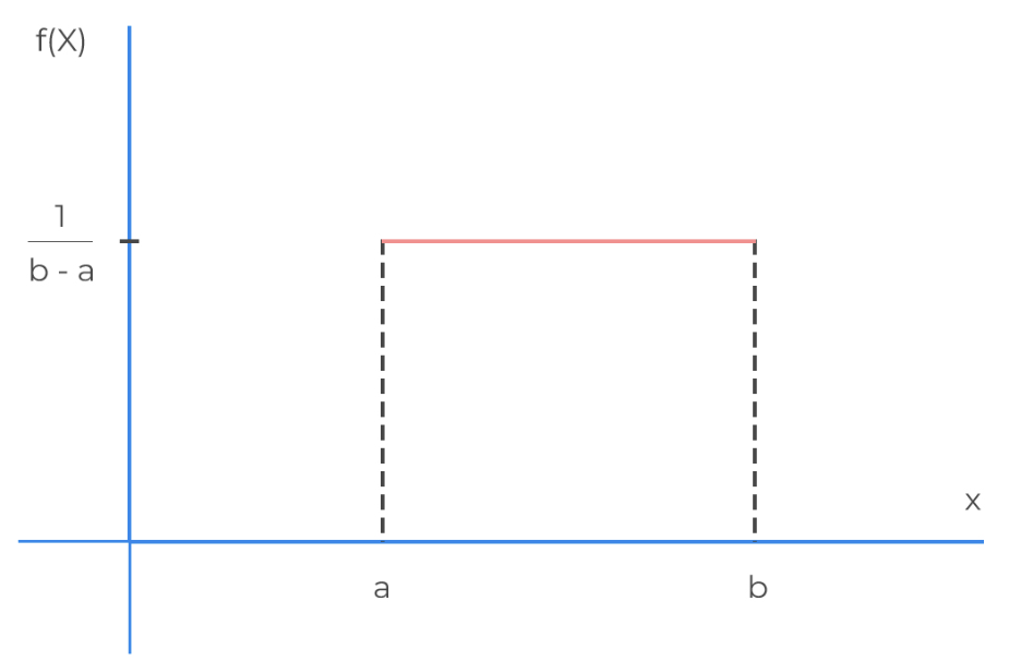
Uniform\[\small f_X(x) = \begin{cases} \frac {1}{b-a} &\text{if } a \le x \le b \\ 0 &\text{otherwise} \end{cases}\]

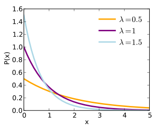
Exponential\[\small f_X(x) = \begin{cases} \lambda e^{-\lambda x} &\text{if } x \ge 0 \\ 0 &\text{otherwise} \end{cases}\]

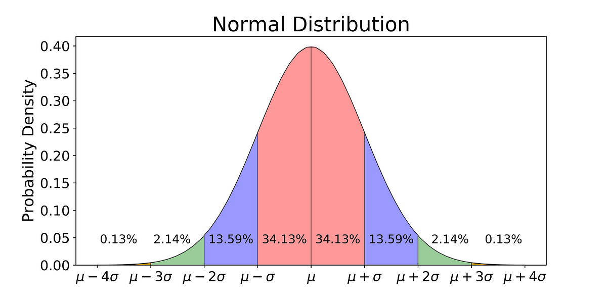
Gaussian\[f_X(x) = \frac {1} {\sqrt{2 \pi} \ \sigma} e^{ \frac{1}{2} (\frac {x-\mu}{\sigma})^2}\]

Working with multiple variables

So, we have now mastered dealing with probabilities involving a single variable. But, the beautiful concept of demystifying uncertainty can be applied to model the “highly random” real world. However, we first need to learn to deal with two variables. Only then can we completely model the real world, which contains so many variables. Let’s dive right in, shall we?

Joint CDF and Marginal CDF

Working with two variables means analysing their probability distribution together. Let our variables be \(X\) and \(Y\). Then, the joint cumulative function can be quite analogously defined as: \[F_{XY} (x, y) = P(X \le x, Y \le y)\] Great! But, we may also want to observe just one variable. Given the joint CDF, we can easily do that as follows: \[F_{X} (x) = \lim\limits_{y \rightarrow \infty} F_{XY} (x, y)\] These are called the marginal cumulative distribution functions. Here, the logic behind \(y \rightarrow \infty\) and \(x \rightarrow \infty\) is to allow all values of that variable, which ensures that the existence of that variable is being fully considered.

Some properties of joint CDF include:

\(\lim\limits_{x, y \rightarrow -\infty} F_{XY} (x, y) = 0\)
\(\lim\limits_{x, y \rightarrow \infty} F_{XY} (x, y) = 1\)

Joint PMF and Marginal PMF

For two discrete random variables \(X\) and \(Y\), we can simply define the joint probability mass function as: \[p_{XY}(x, y) = P(X=x, Y=y)\] Let the set of all possible values taken by \(X\) and \(Y\) be \(Val(X)\) and \(Val(Y)\). Quite easily, the marginal probability mass function can be said to be: \[p_X(x) = \sum_{y \in Val(Y)} p_{XY}(x, y)\]

Joint PDF and Marginal PDF

If the joint CDF is differentiable everywhere, we can define the joint probability density function as follows: \[f_{XY}(x, y) = \frac {\partial^2 F_{XY}(x, y)} {\partial x \partial y}\] Similarly, we can define the marginal probability density function as: \[f_X(x, y) = \int_{-\infty}^{\infty} f_{XY}(x, y)dy\] Also, \[\int_{-\infty}^{\infty} \int_{-\infty}^{\infty} f_{XY} (x, y) dxdy = 1\]

Expectation and Covariance

For discrete variables, \[\mathbb{E}[g(X, Y)] = \sum_{x \in Val(X)} \sum_{y \in Val(Y)} g(x, y)p_{XY}(x, y)\] For continuous variables, \[\mathbb{E}[g(X, Y)] = \int_{-\infty}^{\infty} \int_{-\infty}^{\infty} g(x, y)f_{XY}(x, y)dxdy\] Now, a useful thing to observe is how both variables “correlate” with each other. By “correlate”, I mean “do larger values of \(X\) correspond with larger values of \(Y\) and how often?”. This is called covariance and can be computed as follows: \[Cov[X, Y] = \mathbb{E} [(X - \mathbb{E}[X])(Y-\mathbb{E}[Y])]\] By a little manuevering, we can derive: \[Cov[X, Y] = \mathbb{E}[XY] - \mathbb{E}[X]\mathbb{E}[Y]\] When larger values of \(X\) correspond with larger values of \(Y\), the covariance is negative. On the other hand, when larger values of \(X\) correspond with smaller values of \(Y\), the covariance is positive.

Some important points to note:

\(Var[X + Y] = Var[X] + Var[Y] + 2Cov[X, Y]\)
\(Cov[X, Y]=0 \rightarrow\) Independence of \(X\) and \(Y\) but its inverse is not true. A counter-example is: Take \(X\) and \(Y\) such that \(Y=X^2\). Here, \(Cov[X, Y] = 0\) but \(X\) and \(Y\) are clearly not independent.

Conditional Probability

Let \(A\) and \(B\) be two events. The probability of an event \(A\) after observing the occurrence of the event \(B\) is termed as conditional probability and denoted by \(P(A | B)\). If \(P(B) \ne 0\), we can define the conditional probability as: \[P(A | B) = \frac {P(A \cap B)}{P(B)}\] The logic behind this famous problem is not that famous, unfortunately! Let me explain. Let \(S\) be the sample space. Our task is to find the probability of \(A\) given that we have observed \(B\). Obviously, \(P(S) = 1\). However, we need to focus on \(B\) which is a subset of \(S\). So, we need to define another function \(P^\prime\) such that \(P^\prime (B) = 1\). This leads us to the following definition of \(P^\prime\): \[P^\prime(A) = \frac {1}{P(B)} P(A)\] However, there’s a small catch. Since we have observed \(B\), we need to discard the part of \(A\) which resides outside of \(B\)! Hence, the new definition becomes: \[P^\prime(A) = \frac {1}{P(B)} P(A \cap B)\]

The Concept of Independence

Only a bit of common sense is required to understand that \(A\) and \(B\) are independent if: \[P(A|B) = P(A)\] Putting in the conditional probability formula, we get: \[P(A \cap B) = P(A) \cdot P(B)\]

The Laws and Rules

Law of Total Probability

If \(A_1, A_2, ..., A_k\) are a set of disjoint events such that \(\bigcup_i A_i = \varOmega\) , then \(\sum_{i=1}^kP(A_i)=1\).

Chain Rule

\(p_{X_1, \ldots ,X_n}(x_1, \ldots , x_n) = p_{X_1}(x_1) \cdot p_{X_2 | X_1}(x_2 | x_1) \cdots p_{X_n | X_1, \ldots X_{n-1}}(x_n | x_1, \ldots x_{n-1})\)

Bayes’ Rule

Quite often, it is easy to know about the dependency of effect on the cause. However, the reverse task is quite harder. Here, the Bayes’ theorem comes into play.

We already know that, \[P(A | B) = \frac {P(A \cap B)}{P(B)} \ and \ P(B | A) = \frac {P(A \cap B)}{P(A)}\] Eliminating \(P(A \cap B)\), we get, \[P(A | B) = \frac {P(B|A) \cdot P(A)}{P(B)}\]

Conclusion

Several concepts, ranging from the basic cross-entropy loss to an advanced architecture like the variational autoencoder, require a clear understanding of this beautiful branch of mathematics. Rest assured! Now, you are well-equipped in terms of probability-related concepts and ready to dive straight into the world of neural networks. I have tried my best to pour this knowledge into a clear, jargon-less language. I hope it helps!

Thanks a lot for reading such a long blog. It took me a lot of hours to put it here, and I would appreciate your feedback. If you find a mistake, feel free to comment or send an email to shah.15@iitj.ac.in. I will be posting new blogs related to deep learning in the upcoming days. Stay tuned!