What is Generative Modelling?
Generative modelling is the task of modelling the data distribution (which helps us generate new, similar, synthetic data points). There are multiple ways of dealing with this problem, with VAEs, diffusion models, and GANs being some of the popular ones. RBMs belong to this category of generative models, i.e. they are trained to model the data distribution \(p(x)\).
In this blog, we will extensively explore binary RBMs (i.e., RBMs that support only binary data). RBMs are not used today because training them on continuous data is difficult. Nevertheless, I find them to be a great introduction to energy-based models and concepts like Gibbs sampling and the Gibbs-Boltzmann distribution. Let’s start right away.
The Concept of Energy
Today, there exists a class of models called energy-based models, which provide a physics-oriented approach to model complex probability distributions based on the concept of “energy” of a system. This is made possible by defining an energy function \(E(\phi)\) which calculates the energy of a given state \(\phi\). Utilising \(E(\phi)\), we can project the energy to a probabilistic space by using the Gibbs-Boltzmann distribution so that lower-energy states will have higher probability density and vice versa.
\[ p(\phi) = \frac{1}{Z} e^{-E(\phi)} ; \text{ where } Z = \sum_{\phi} e^{-E(\phi)} \text{ is a normalising factor} \]
Architecture
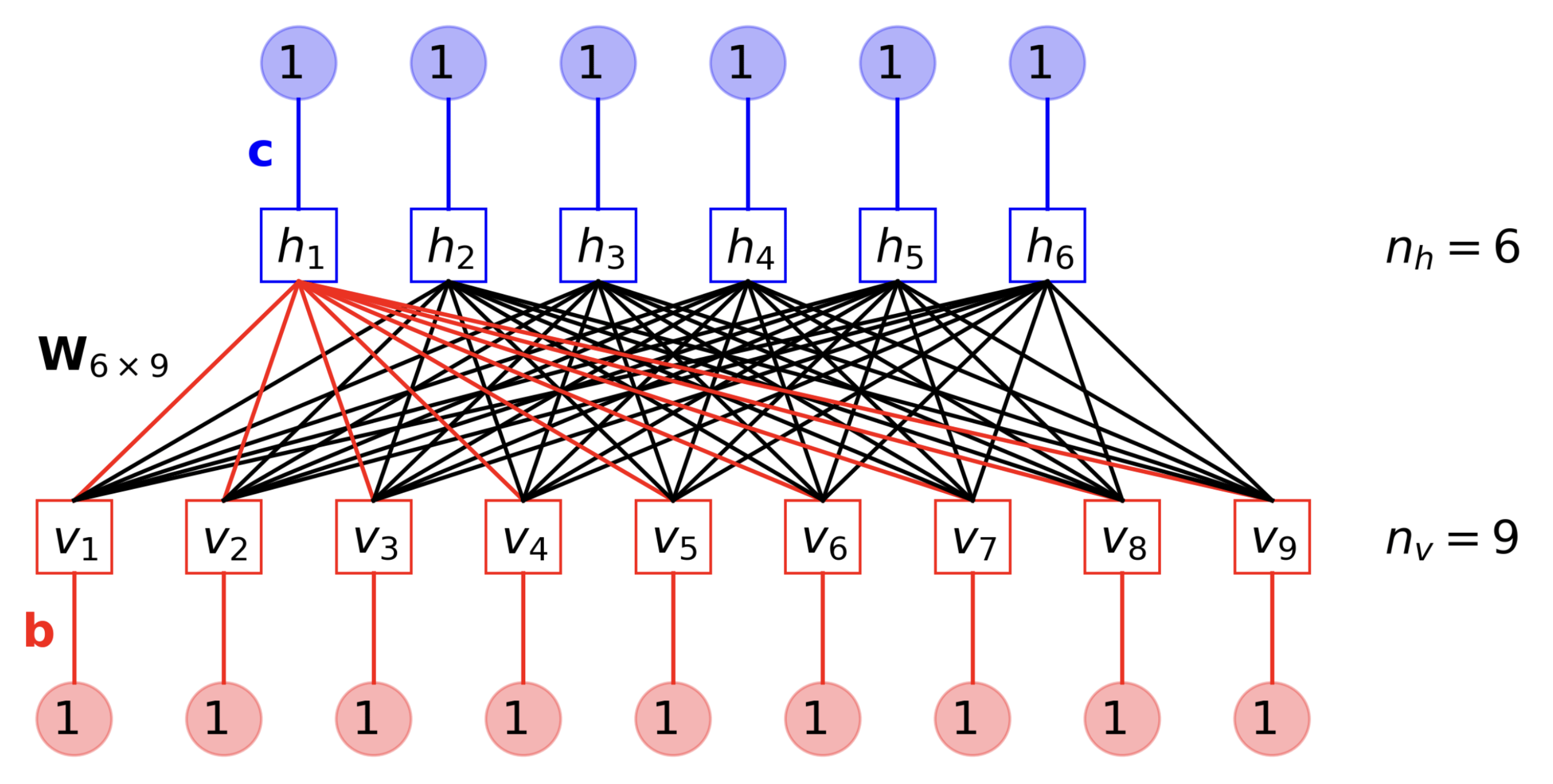
The components of binary RBMs can be separated into:
State
- Visible Nodes - These binary nodes are responsible for representing the data points in the input space. The use of these nodes will be clearer as we go deeper.
- Hidden Nodes - These are binary nodes responsible for creating an information bottleneck to enforce proper learning of underlying features. They represent data points in the latent space.
Learnable Parameters
- Visible Biases - Each of the visible nodes has a bias parameter.
- Hidden Biases - Each of the hidden nodes has a bias parameter.
- Weights - Each visible node is connected to all hidden nodes through learnable weights. Basically, these weights will be a matrix of size (num_visible_nodes x num_hidden_nodes).
Notation
\(m\) - number of visible nodes
\(v_j\) - \(j^{th}\) visible node
\(b_j\) - bias of \(j^{th}\) visible node
\(\textbf{v}\) - \([v_1, \dots v_m]\)
\(n\) - number of hidden nodes
\(h_i\) - \(i^{th}\) hidden node
\(c_i\) - bias of \(i^{th}\) hidden node
\(\textbf{h}\) - \([h_1, \dots h_n]\)
\(w_{ij}\) - weight connecting the \(j^{th}\) visible node and the \(i^{th}\) hidden node
Log-Likelihood
Like every other generative model, RBMs are trained to learn a probability distribution to maximise the probability (or the log probability) of observing the observed training samples. In other words, assuming only one sample \(\textbf{v}\) is given, we need to find theta such that the below function is maximised:
\[ \mathcal{L}(\theta|\textbf{v}) = ln(p(\textbf{v}|\theta)) \]
Here’s where the energy-based approach comes into play by providing a platform to define \(p(\textbf{v})\). The energy function for RBMs is defined as:
\[ E(\textbf{v}, \textbf{h}) = - \sum_{i} \sum_{j} w_{ij} v_j h_i - \sum_{j} b_j v_j - \sum_{i} c_i h_i \]
Given the weights and biases, this energy function measures the compatibility between the visible and hidden units. Lower energy states correspond to more compatible or favourable configurations of visible and hidden units, while higher energy states correspond to less compatible configurations.
Since we now have the energy function, we can calculate the joint probability distribution as:
\[ p(\textbf{v}, \textbf{h}) = \frac{1}{Z} e^{-E(\textbf{v}, \textbf{h})} \]
Where \(Z = \sum_{\textbf{v}, \textbf{h}} e^{-E(\textbf{v}, \textbf{h})}\) the normalisation constant (also known as the partition function) ensures that the probabilities sum up to 1 over all possible configurations.
Defining the joint distribution unlocks the ability to define all underlying distributions. Through a series of calculations, we get the following expressions:
The joint distribution can now be used to define \(p(\textbf{v})\), the logarithm of which we need to minimise.
\[ p(\textbf{v}) = \sum_\textbf{h} p(\textbf{v}, \textbf{h}) = \frac{1}{Z} \sum_\textbf{h} e^{-E(\textbf{v}, \textbf{h})} \]
Since \(\textbf{h}\) is a binary variable, it can be represented with the help of a Bernoulli distribution as follows:
\[ p(H_i=1| \textbf{v}) = \sigma \Big(\sum_{j=1}^m w_{ij}v_j + c_i \Big) \\ p(H_i=0| \textbf{v}) = 1 - p(H_i=1| \textbf{v}) \]
Since \(\textbf{v}\) is also a binary variable, so we can do the same here as well:
\[ p(V_j=1| \textbf{h}) = \sigma \Big(\sum_{i=1}^n w_{ij}h_i + b_j \Big) \\ p(V_j=0| \textbf{h}) = 1 - p(V_j=1| \textbf{h}) \]
Gradient Calculation Logic
Let’s go through a clear breakdown of the differentiation process. First, let’s simplify the loss function a bit:
\[\begin{equation*} \begin{split} \mathcal{L}(\theta|\textbf{v}) &= ln(p(\textbf{v}|\theta)) = ln \Big(\frac{1}{Z} \sum_\textbf{h} e^{-E(\textbf{v}, \textbf{h})} \Big) \\ &= ln \Big(\sum_\textbf{h} e^{-E(\textbf{v}, \textbf{h})} \Big) - ln(Z) \\ &= ln \Big(\sum_\textbf{h} e^{-E(\textbf{v}, \textbf{h})} \Big) - ln \Big(\sum_{\textbf{v}, \textbf{h}} e^{-E(\textbf{v}, \textbf{h})} \Big) \end{split} \end{equation*}\]
Using the simple chain rule, we can calculate the gradient as follows:
\[\begin{equation*} \begin{split} \frac{\partial\mathcal{L}(\theta|\textbf{v})}{\partial \theta} &= \frac{\partial}{\partial \theta} \Big( ln \Big(\sum_\textbf{h} e^{-E(\textbf{v},\textbf{h})} \Big) \Big) - \frac{\partial}{\partial \theta} \Big( ln \Big(\sum_{\textbf{v},\textbf{h}} e^{-E(\textbf{v},\textbf{h})} \Big) \Big) \\ &= - \frac{1}{\sum_\textbf{h} e^{-E(\textbf{v},\textbf{h})}} \sum_\textbf{h} e^{-E(\textbf{v},\textbf{h})} \frac{\partial E(\textbf{v},\textbf{h})}{\partial \theta} + \frac{1}{\sum_{\textbf{v},\textbf{h}} e^{-E(\textbf{v},\textbf{h})}} \sum_{\textbf{v},\textbf{h}} e^{-E(\textbf{\textbf{v},\textbf{h}})} \frac{\partial E(\textbf{v},\textbf{h})}{\partial \theta} \end{split} \end{equation*}\]
Now, we already know that,
\[ p(\textbf{v},\textbf{h}) = \frac{e^{-E(\textbf{v},\textbf{h})}}{\sum_{\textbf{v},\textbf{h}} e^{-E(\textbf{v},\textbf{h})}} \]
\[ p(\textbf{h}|\textbf{v}) = \frac{p(\textbf{v},\textbf{h})}{p(\textbf{v})} = \frac{\frac{1}{Z} e^{-E(\textbf{v},\textbf{h})}}{\frac{1}{Z} \sum_\textbf{h} e^{-E(\textbf{v},\textbf{h})}} = \frac{ e^{-E(\textbf{v},\textbf{h})}}{\sum_\textbf{h} e^{-E(\textbf{v},\textbf{h})}} \]
Therefore, we can just put these in the gradient equation as follows:
\[\begin{equation*} \begin{split} \frac{\partial\mathcal{L}(\theta|\textbf{v})}{\partial \theta} &= - \sum_\textbf{h} p(\textbf{h}|\textbf{v}) \frac{\partial E(\textbf{v},\textbf{h})}{\partial \theta} + \sum_{\textbf{v},\textbf{h}} p(\textbf{v},\textbf{h}) \frac{\partial E(\textbf{v},\textbf{h})}{\partial \theta} \end{split} \end{equation*}\]
Gradient Calculation for \(w_{ij}\)
Now, we will look at the simplification of the gradient of loss w.r.t the weights (i.e. \(\theta = w_{ij}\)).
First Term Simplification
Now, let’s calculate the first term of this gradient with \(\theta\) as \(w_{ij}\):
\[ -\sum_\textbf{h} p( \textbf{h | v} ) \frac{\partial E(\textbf{v}, \textbf{h})}{\partial w_{ij}} = \sum_\textbf{h} p( \textbf{h | v} ) h_i v_j \]
Here, some calculation tricks can be applied to simplify the right-side expression:
- Since, all \(h_i\)’s are independent, we can write \(p( \textbf{h | v} ) = \prod_{k=1}^n p(h_k|\textbf{v})\).
- \(\sum_h\) can be rewritten as \(\sum_{h_i} \sum_{\textbf{h}_{\textbf{-i}}}\), where \(\textbf{h}_{\textbf{-i}}\) represents a vector without the ith node.
- Lastly, we can rewrite \(\prod_{k=1}^n p(h_k|\textbf{v}) = p(h_i| \textbf{v}) p(\textbf{h}_{\textbf{-i}} | \textbf{v})\).
- \(\sum_{\textbf{h}_{\textbf{-i}}} p(\textbf{h}_{\textbf{-i}} | \textbf{v}) = 1\), obviously!
Using the above tricks, the equation becomes:
\[\begin{equation*} \begin{split} -\sum_\textbf{h} p( \textbf{h | v} ) h_i v_j &= \sum_{h_i} \sum_{\textbf{h}_{\textbf{-i}}} p(h_i| \textbf{v}) p(\textbf{h}_{\textbf{-i}} | \textbf{v}) h_i v_j \\ &= \sum_{h_i} p(h_i| \textbf{v}) h_i v_j \sum_{\textbf{h}_{\textbf{-i}}} p(\textbf{h}_{\textbf{-i}} | \textbf{v}) \\ &= \sum_{h_i} p(h_i| \textbf{v}) h_i v_j \\ &= p(H_i=0| \textbf{v}) (0) v_j + p(H_i=1| \textbf{v}) (1) v_j \\ &= p(H_i=1| \textbf{v}) v_j \\ &= \sigma \Big(\sum_{j=1}^m w_{ij}v_j + c_i \Big) v_j \end{split} \end{equation*}\]
Second Term Simplification
\[\begin{equation*} \begin{split} \sum_{\textbf{v},\textbf{h}} p(\textbf{v},\textbf{h}) \frac{\partial E(\textbf{v},\textbf{h})}{\partial w_{ij}} &= -\sum_\textbf{v} p(\textbf{v}) \sum_\textbf{h} p( \textbf{h | v} ) h_i v_j \\ &= -\sum_\textbf{v} p(\textbf{v}) p(H_i=1| \textbf{v}) v_j \end{split} \end{equation*}\]
Hence, the final gradient comes out to be:
\[ \frac{\partial\mathcal{L}(\theta|\textbf{v})}{\partial w_{ij}} = p(H_i=1| \textbf{v}) v_j - \sum_\textbf{v} p(\textbf{v}) p(H_i=1| \textbf{v}) v_j \]
Final Gradient Calculation Formulas
Similar to what we did for \(w_{ij}\), we can calculate the gradient formulae for \(b_j\) and \(c_i\). Hence, the final gradients formulae are:
\[ \frac{\partial\mathcal{L}(\theta|\textbf{v})}{\partial w_{ij}} = p(H_i=1| \textbf{v}) v_j - \sum_\textbf{v} p(\textbf{v}) p(H_i=1| \textbf{v}) v_j \]
\[ \frac{\partial\mathcal{L}(\theta|\textbf{v})}{\partial b_{j}} = v_j - \sum_\textbf{v} p(\textbf{v}) v_j \]
\[ \frac{\partial\mathcal{L}(\theta|\textbf{v})}{\partial b_{j}} = p(H_i=1| \textbf{v}) - \sum_\textbf{v} p(\textbf{v}) p(H_i=1| \textbf{v}) \]
Approximating the Gradients
There’s a big problem with the above equations. Looping over \(\textbf{v}\) is intractable. However, we can estimate this expectation with a series of approximations.
Approx. 1
Instead of looping over \(\textbf{v}\), we sample some samples from the distribution at hand [\(p(\textbf{v}, \textbf{h})\) in this case] and calculate their mean. Practically, using just one sample works fine and fairly approximates the expectation.
\[ \hat{\textbf{v}} \sim p(\textbf{v}, \textbf{h}) \]
\[ \frac{\partial\mathcal{L}(\theta|\textbf{v})}{\partial w_{ij}} = p(H_i=1| \textbf{v}) v_j - p(H_i=1| \hat{\textbf{v}}) \hat{v}_j \]
\[ \frac{\partial\mathcal{L}(\theta|\textbf{v})}{\partial b_{j}} = v_j - \hat{v}_j \]
\[ \frac{\partial\mathcal{L}(\theta|\textbf{v})}{\partial b_{j}} = p(H_i=1| \textbf{v}) - p(H_i=1| \hat{\textbf{v}}) \]
Approx. 2
Still, sampling \(\hat{\textbf{v}}\) from \(p(\textbf{v}, \textbf{h})\) is not possible because of the intractable \(Z\) term encountered in the calculation of \(p(\textbf{v}, \textbf{h})\). However, the good news is that it is relatively (very!) easy to calculate \(p(\textbf{h} | \textbf{v})\) and \(p(\textbf{v} | \textbf{h})\) (remember the Bernoulli distributions we described a while ago?). Here’s where the Gibbs sampler comes in handy.
Basically, according to Mr. Gibbs, if you start with some \(\textbf{v}^0\) AND sample \(\textbf{h}^1 \sim p(\textbf{h} | \textbf{v}^0)\) and \(\textbf{v}^1 \sim p(\textbf{v} | \textbf{h}^1)\) AND keep going till convergence (suppose we reach convergence after \(k\) iterations), the samples \(\textbf{h}^k\) and \(\textbf{v}^k\) will look as if they were sampled from the intractable joint distribution \(p(\textbf{v}, \textbf{h})\).
We use Gibbs sampling because we can easily sample from \(p(\textbf{h}|\textbf{v})\) and \(p(\textbf{v}|\textbf{h})\) which are simple Bernoulli distributions.
Approx. 3
A small problem persists — performing Gibbs sampling until convergence is computationally expensive. However, the good news is that performing just one step of Gibbs sampling approximates the sampling process fairly enough for the gradient descent algorithm to work.
Final Algorithm
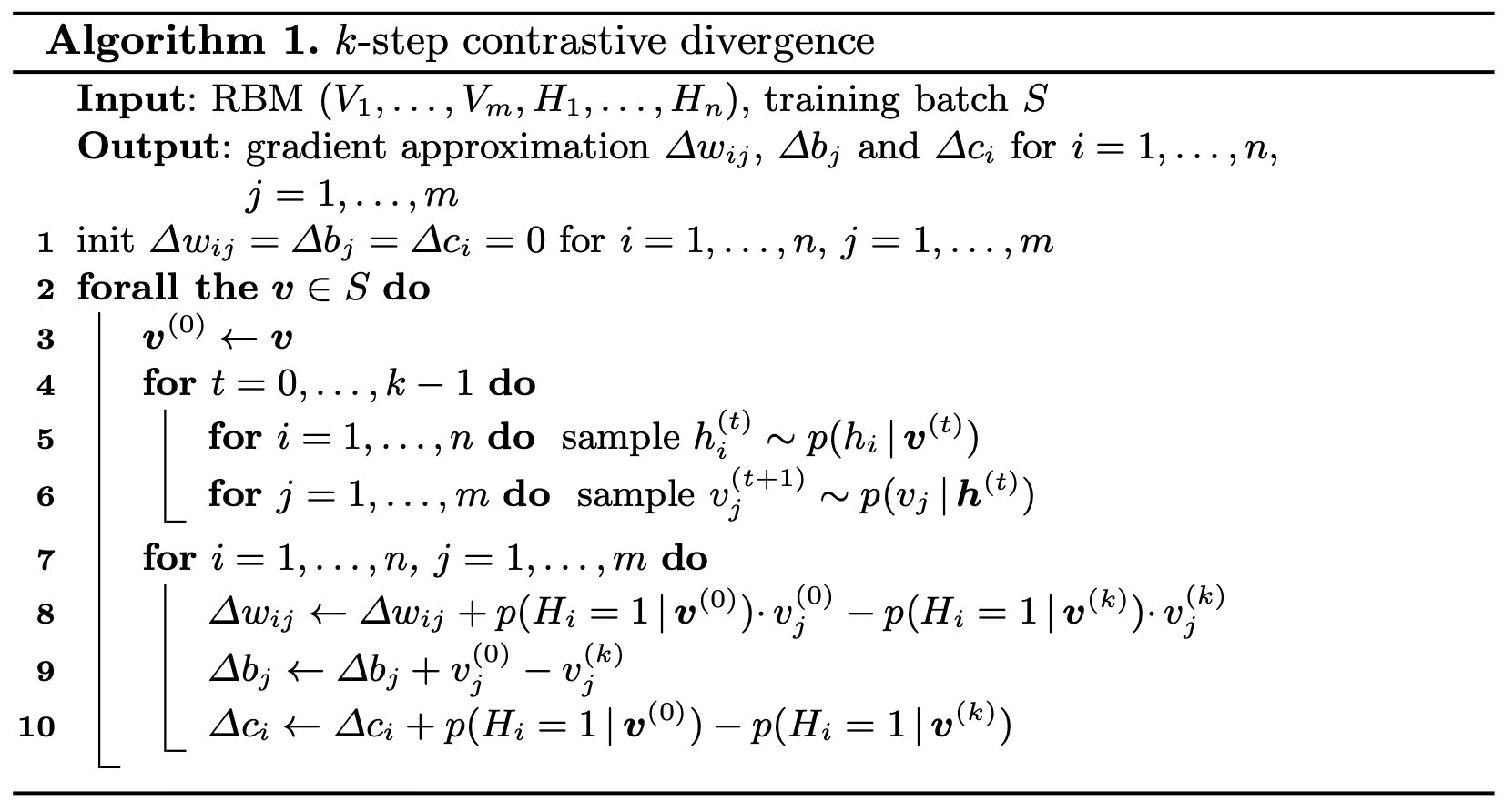
All the above approximations combine to form the “Contrastive Divergence” algorithm for calculating the gradients of an RBM, which is seen clearly as follows:
The above algorithm can be broken down as follows:
- Initialise variables to store the gradient approximations. These will be used to update the parameters using gradient ascent.
- Iterate over the training set and:
- Get a good approximation of a sample from the joint distribution by performing k iterations of Gibbs sampling.
- Calculate the gradient of each parameter using the formulae we derived earlier.
- Use the gradient storage variables to accumulate gradients for each parameter by adding the calculated gradient.
- The final value of these gradient storage variables will be the final gradient approximation.
- (Not mentioned in the above photo) Using the gradient approximations outputted above, update the parameters using gradient ascent(we are maximising the \(\mathcal{L}(\theta|\textbf{v})\), hence ascent).
With this, we have finally completed learning about binary RBMs. A lot of math, wasn’t it? I tried to make it as clear as possible, but if you have suggestions, feel free to contact me on shahrushi2003@gmail.com.

